Advanced Visualizations#
Density plots, heatmaps, and joint distributions for in-depth shot pattern analysis.
KDE (Kernel Density Estimation)#
Smooth contour plots showing shot concentration.
Green |
Red |
Blue |
|---|---|---|
|
|
|
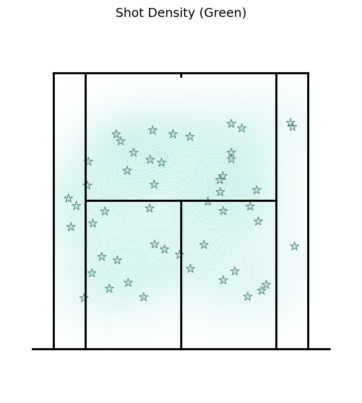
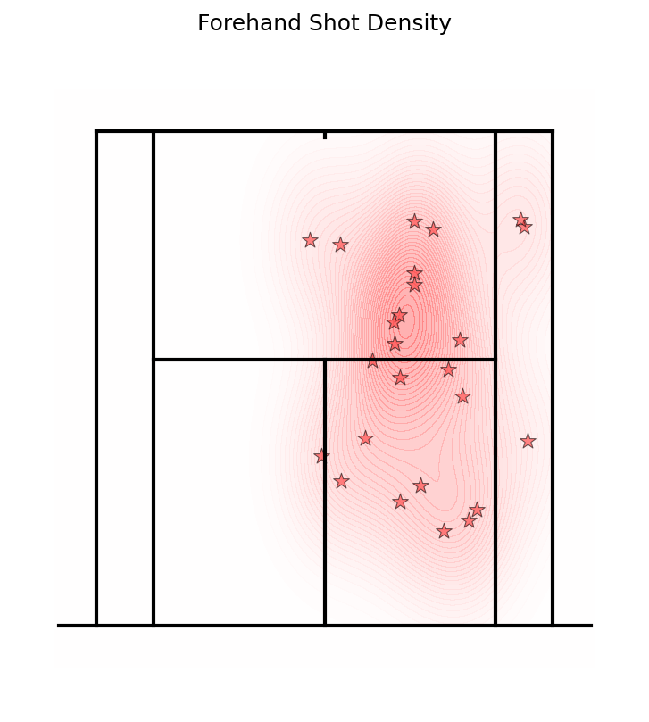
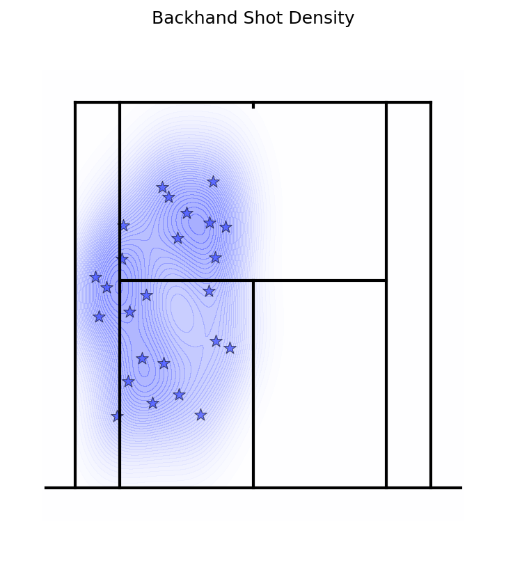
court.kdeplot(ax, x, y, cmap='bsu_green', levels=50, alpha=0.6)
Colormaps: bsu_green, bsu_red, bsu_blue
Heatmap (Grid)#
Frequency distribution across grid cells.
Counts |
Frequency (%) |
|---|---|
|
|
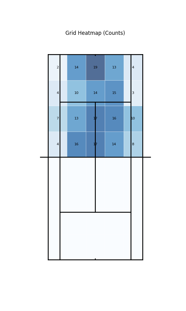
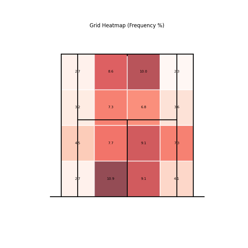
court.heatmap(ax, x, y, gridsize=8, statistic='frequency', half=True)
Hexbin#
Honeycomb-style density visualization.
Full Court |
Half Court |
|---|---|
|
|
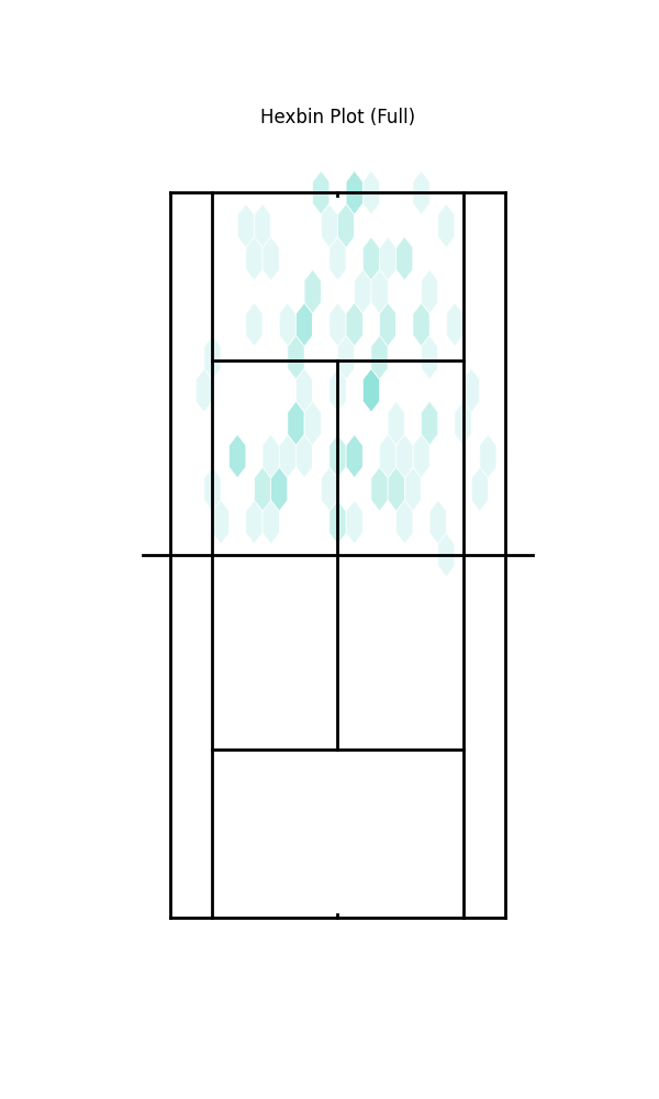
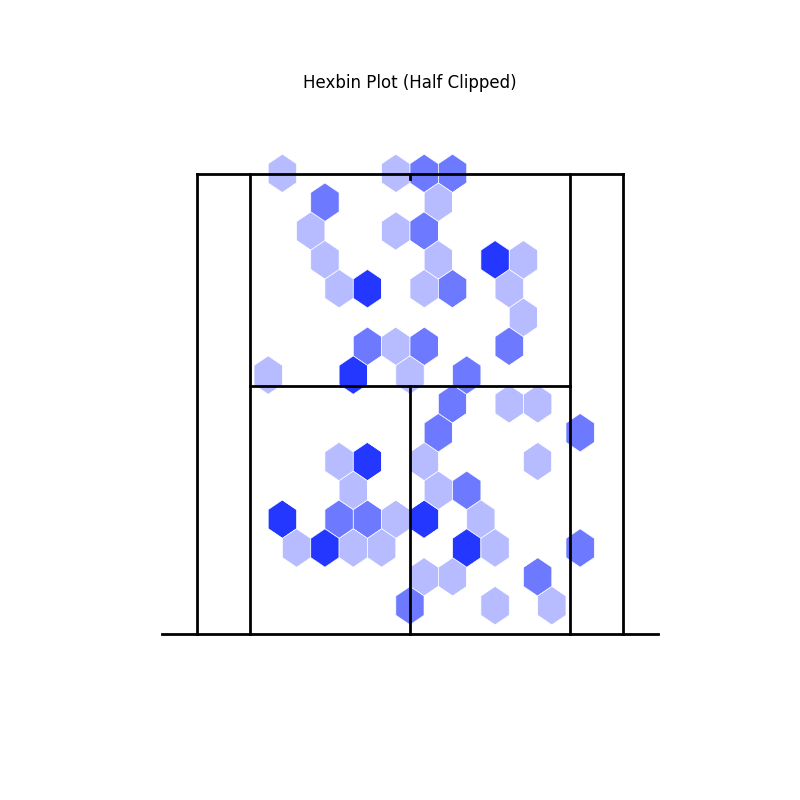
court.hexbin(ax, x, y, gridsize=20, cmap='bsu_green', half=True)
Sonar Chart#
Shot direction distribution from court zones.
6-Direction |
8-Direction |
Custom |
|---|---|---|
|
|
|
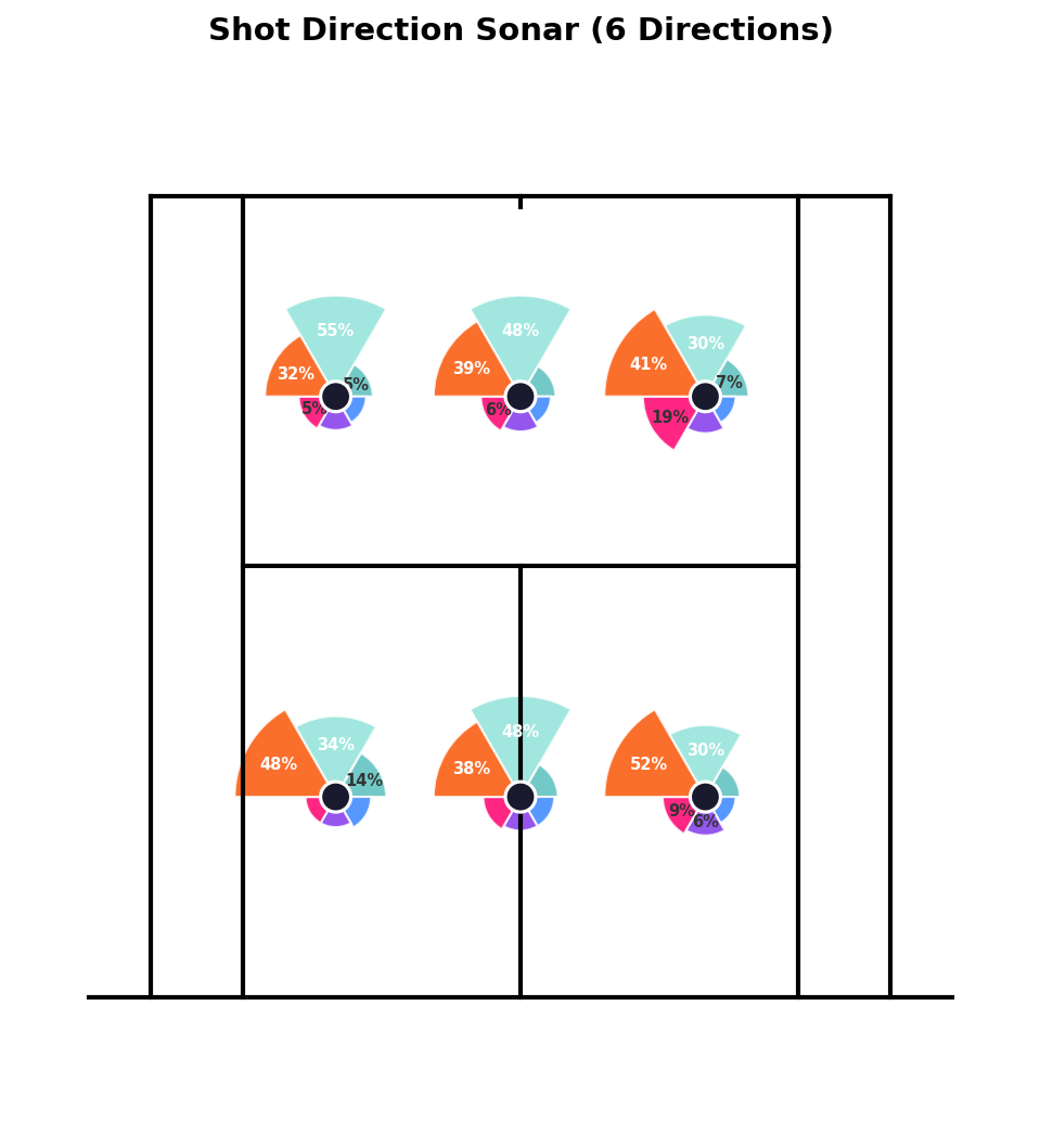
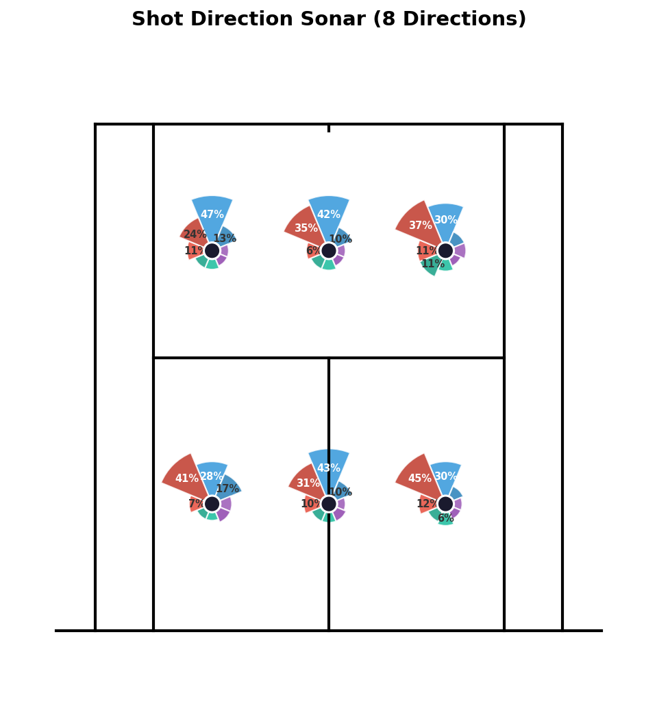
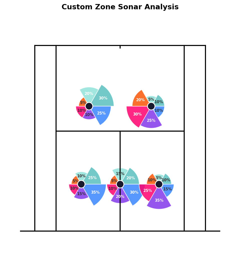
from BsuTennis import sonar_from_shots

sonar_from_shots(ax, shot_x, shot_y, shot_dx, shot_dy,
                 n_zones_x=3, n_zones_y=2, n_directions=6)
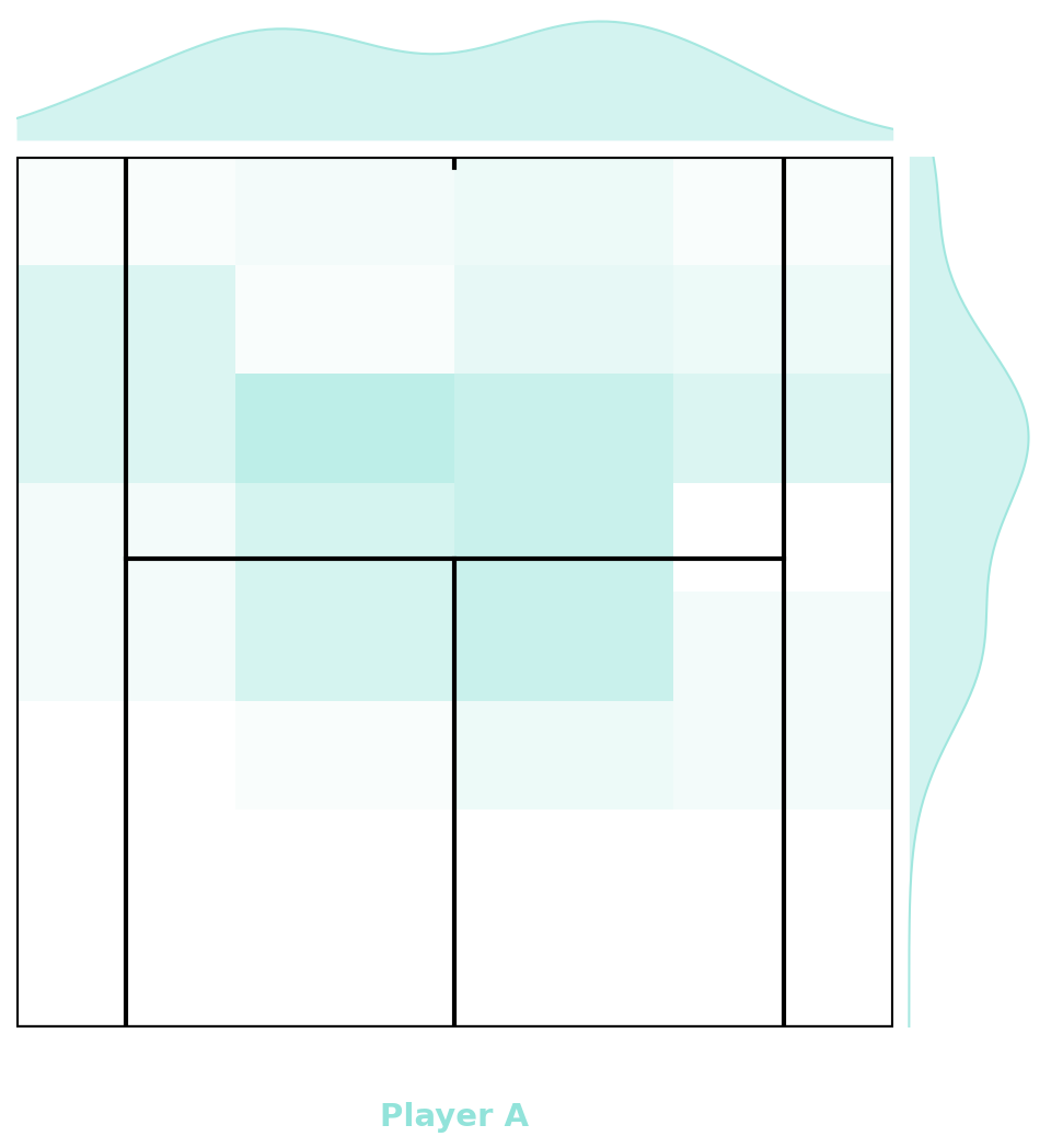
Joint Plots#
Court visualization with marginal distributions.
Full Court (Two Players)#
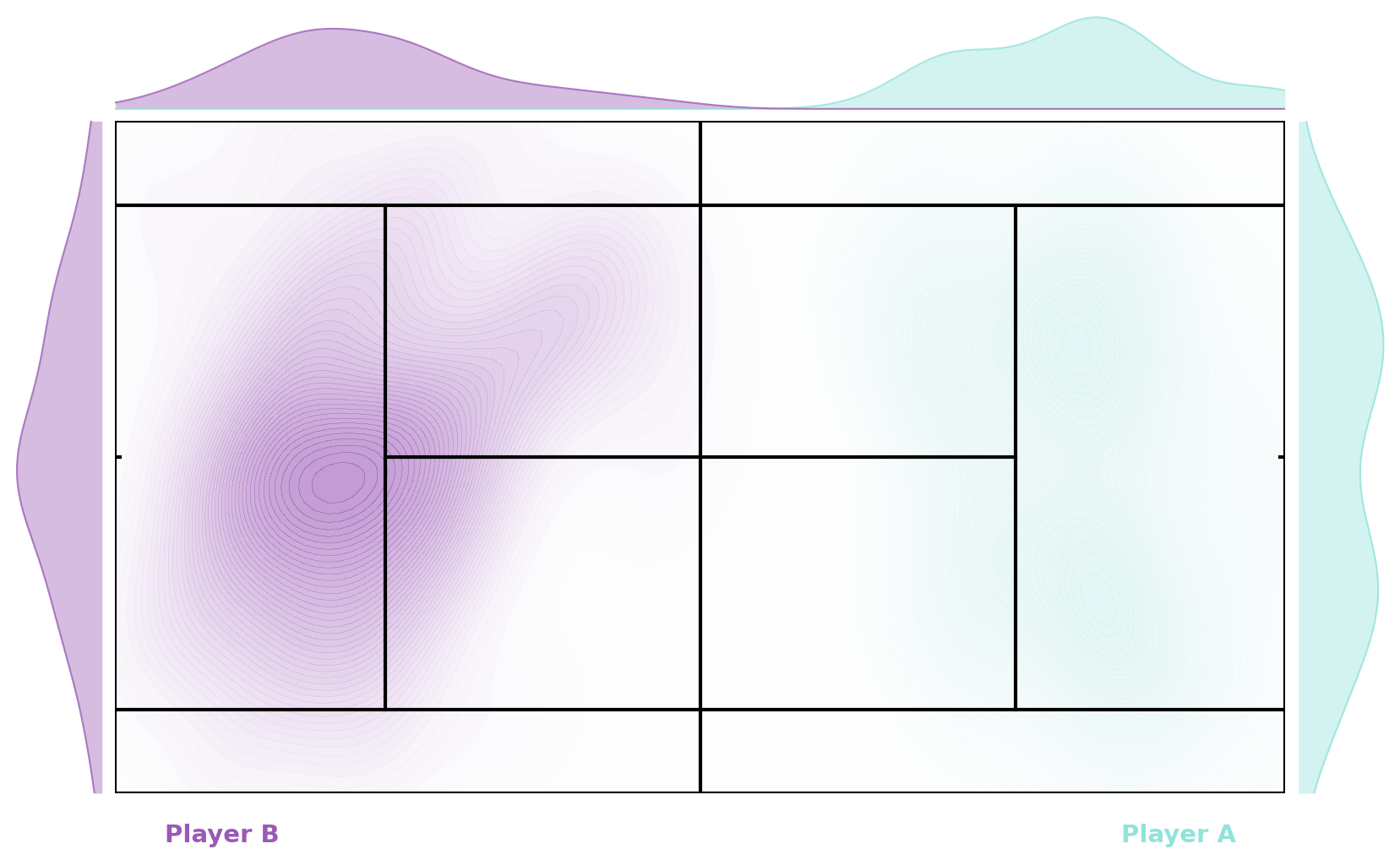
from BsuTennis import joint_plot

fig, ax = joint_plot(p1_x, p1_y, p2_x, p2_y, kind='kde', half=False)
Half Court#
Scatter |
Grid |
|---|---|
|
|
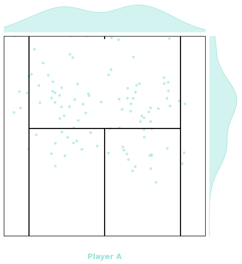
fig, ax = joint_plot(x, y, kind='scatter', half=True)
fig, ax = joint_plot(x, y, kind='grid', half=True)
Types: scatter, kde, grid